10 Excel 2013 Advanced Formulas and Functions: Power Tools for Data Crunching Like a Pro

Tired of VLOOKUP breaking when your data rearranges or needing helper columns for complex lookups? The array formula with INDEX and MATCH is your upgrade path—handling dynamic ranges and multi-criteria searches effortlessly in Excel 2013.

This combo uses INDEX to fetch values and MATCH to locate them, letting you search left-to-right (unlike VLOOKUP’s right-only limitation). Press Ctrl+Shift+Enter to make it an array formula, and it’ll return exact matches even across non-adjacent columns. For example: =INDEX(B:B, MATCH(1, (A:A="Apple")*(C:C="Red"), 0)) finds red apples without extra columns.

Perfect for analysts juggling large datasets with shifting structures—like inventory systems or sales reports where columns frequently reorder. Master this first, and you’ll breeze through the rest. ✨

Tired of manually adjusting ranges every time your financial dataset grows? The OFFSET and COUNTA combo creates dynamic arrays that expand automatically—no helper columns needed. This is Excel 2013’s secret weapon for models where data shifts constantly, like quarterly revenue projections or inventory tracking.

Start with COUNTA to count your data rows, then use OFFSET to reference a range that starts at a fixed cell and extends dynamically. For example, =SUM(OFFSET(A1,0,0,COUNTA(A:A),1)) sums column A while expanding as new entries are added. Combine with INDEX for multi-column flexibility, and you’ve built a self-adjusting range that’s far more reliable than static references.

Financial analysts and small business owners will love this for automated reporting—no more breaking formulas when new data arrives. The best part? It works in Excel 2013’s legacy environment without requiring newer dynamic array functions. ✨

Tired of juggling nested IF statements just to track inventory by category, location, and price range? SUMIFS and COUNTIFS solve this with elegant simplicity—no helper columns required.

These functions let you apply up to 127 conditions simultaneously, whether you're summing sales for red shirts in size M priced under $20 or counting low-stock items across multiple warehouses. The syntax is straightforward: =SUMIFS(sumrange, criteriarange1, criteria1, ...). For inventory managers, this means instant visibility into multi-criteria trends without manual filtering.

Small business owners and warehouse teams will love how these functions replace error-prone manual calculations with bulletproof accuracy. Perfect for scenarios where multiple criteria must align—like tracking seasonal inventory or analyzing regional sales patterns. ✨

Cleaning up messy text data in Excel 2013 just got easier with TEXTJOIN and TRIM. These functions work together to combine text from multiple cells while automatically skipping errors and removing extra spaces—perfect for merging customer feedback or product descriptions scattered across columns.

The TEXTJOIN function lets you specify a delimiter (like commas or spaces) and ignore empty or error cells with its ignoreempty and ignoreerr parameters. Pair it with TRIM to remove leading/trailing spaces from each cell before joining. For example, =TEXTJOIN(", ", TRUE, TRIM(A1:A10)) turns messy data into a polished, error-free string in seconds.

Small business owners and marketers will love this combo for consolidating survey responses or product descriptions. It’s also a lifesaver when merging data from different sources without manual cleanup. ✨

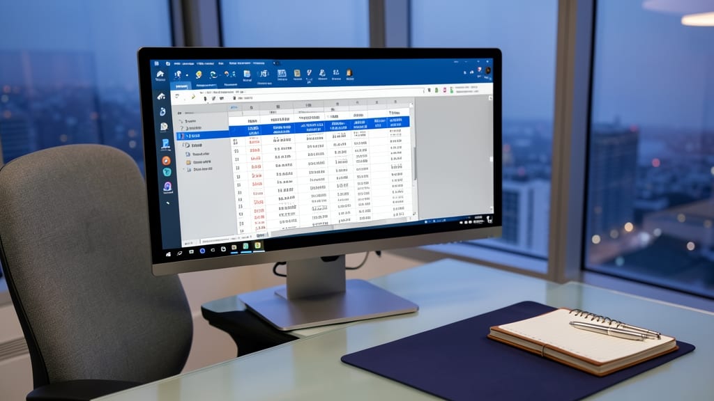
Tracking project timelines or lease durations in Excel 2013 just got easier with DATEDIF and EOMONTH—two functions that handle date math where simple subtraction falls short.

DATEDIF calculates precise differences between dates in years, months, or days (e.g., =DATEDIF(startdate, enddate, "m") for months), while EOMONTH returns the last day of a month (e.g., =EOMONTH("1/15/2023", 2) yields 3/31/2023). Together, they solve common pain points like partial-month billing or milestone tracking without manual adjustments. ⚡

Project managers and financial analysts will love these for automating deadlines and calculating exact durations—no more guessing or rounding errors. 💻

Quality control teams often struggle to validate process capability without diving into manual sorting—PERCENTILE and QUARTILE in Excel 2013 solve this by revealing data distribution patterns instantly.

Use PERCENTILE.INC to pinpoint exact thresholds (e.g., the 90th percentile for defect rates) or QUARTILE.INC to split data into four equal parts for quick trend analysis. These functions work on unsorted data, saving hours of manual work. For example, =QUARTILE.INC(A2:A100,2) instantly reveals the median (Q2) of your measurements.

Perfect for manufacturers validating production consistency or analysts spotting outliers in performance metrics—no sorting required! ✨

Financial models and complex calculations can crash hard when errors like #DIV/0! or #VALUE! appear—but IFERROR and ISERROR act as your safety net. These functions quietly catch and handle errors before they disrupt your entire analysis, ensuring clean outputs even when inputs fail.

The IFERROR function lets you specify a fallback value (like "N/A" or zero) when a formula fails, while ISERROR lets you test for errors first. For example, wrap a volatile formula like =A1/B1 in =IFERROR(A1/B1,0) to return zero instead of an error if B1 is blank. Combined, they create bulletproof calculations for scenarios like division by zero or mismatched data types.

Accountants, financial analysts, and anyone working with volatile data will appreciate how these functions preserve workflows without manual error checks. They’re the unsung heroes of Excel 2013’s formula toolkit. ✨

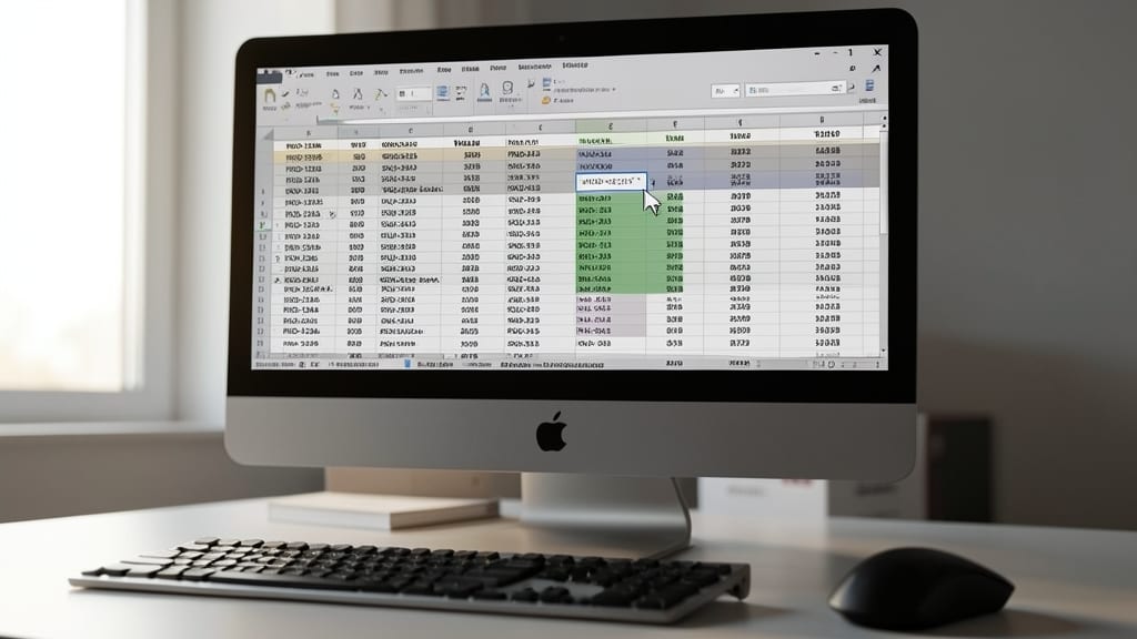
Struggling to find partial product codes in your inventory? VLOOKUP with wildcards was Excel 2013's secret weapon for pattern matching before XLOOKUP arrived. This technique lets you search for text fragments like "PROD-123" or "SKU-2"—perfect when you only remember part of an ID.

Use the wildcard characters (matches any sequence) and ? (matches single characters) in your lookup value. For example, =VLOOKUP("PROD-123", A2:C100, 2, FALSE) instantly pulls all matching inventory items. It’s especially useful for inventory systems where product codes might be mistyped or only partially recalled.

Small business owners and warehouse managers will love this for quick stock checks without manual filtering. It’s the pre-XLOOKUP solution that still holds up today! ✨

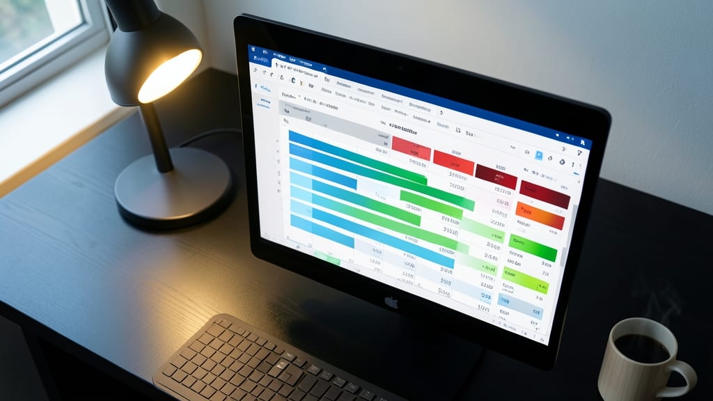
Tired of staring at endless rows of numbers when your sales dashboard could show you the story? Data Bars and Color Scales turn raw data into intuitive visual cues—no charts required. These tools instantly highlight trends, outliers, and performance gaps by filling cells with proportional bars or gradient colors, making patterns obvious at a glance.

With Data Bars, you can display relative values as mini horizontal bars (e.g., green for high, red for low), while Color Scales use a two-color gradient to show data distribution across a range. Both update dynamically as your data changes, and you can customize rules to fit your metrics—like flagging underperforming regions in a red-to-green spectrum or ranking products by sales volume with blue-to-yellow bars.

Perfect for sales teams, project managers, or anyone drowning in KPIs, these features turn passive data into an active dashboard. No more squinting at cells—just instant visual insights that keep your team aligned. ✨

Tired of manually recalculating depreciation schedules every quarter? VBA custom functions let you create reusable, formula-like macros that run directly in your Excel cells—no Alt+F8 required. This is where Excel’s built-in programming meets your financial workflow, turning repetitive tasks into automated precision.

With VBA integration points, you can build functions like DepreciationSchedule() that accept parameters (asset value, life span, method) and return results—just like native Excel functions. The Application.Volatile property ensures your custom functions update automatically when source data changes. For accountants, this means zero manual errors in complex calculations like MACRS or straight-line depreciation.

Perfect for finance teams handling asset registers or tax filings, this approach saves hours weekly while maintaining audit trails. Just enable the Developer tab in Excel 2013 Options, and you’re ready to code your own formulas. ✨